Category:Principal Components Analysis

Principal components analysis identifies interrelationships between variables. In Displayr: Insert > Dimension Reduction > Principal Components Analysis.

Applications of Principal Components Analysis in Survey Analysis

• Understand how attitudes and/or behaviors are interrelated.
• Identify Redundant Questions in a Questionnaire
• Checking Multi-Item Scales (i.e., if the scale has been developed to measure two abstract dimensions using ten variables then principal components analysis should recover these same two dimensions.
• Identify Redundant Concepts in New Product Testing
• Summarize data.
• Transform data prior to the application of other multivariate techniques (e.g., cluster analysis: see Data Preparation for Cluster-Based Segmentation or regression).

An example

The following correlation matrix shows correlations between viewing of a number of different television programs in Britain.^[1] If you inspect the table you will see it reveals some patterns:

• People who watch any one of the sports programs are more likely to watch one of the other sports programs.
• People who watch one current affairs program are more likely to watch another, and vice versa.

	Professional Boxing	This Week	Today	World of Sport	Grandstand	Line-Up	Match of the Day	Panorama	Rugby Special	24 Hours
World of Sport	1.0	.6	.6	.5	.3	.2	.1	.1	.1	.1
Grandstand	.6	1.0	.6	.5	.3	.2	.1	.1	.1	.1
Match of the Day	.6	.6	1.0	.5	.3	.1	.1	.0	.0	.1
Professional Boxing	.5	.5	.5	1.0	.3	.2	.1	.1	.1	.1
Rugby Special	.3	.3	.3	.3	1.0	.1	.1	.1	.1	.1
Panorama	.2	.2	.1	.2	.1	1.0	.5	.2	.2	.4
24 Hours	.1	.1	.1	.1	.1	.5	1.0	.3	.2	.4
Line-Up	.1	.1	.0	.1	.1	.2	.3	1.0	.2	.2
Today	.1	.1	.0	.1	.1	.2	.2	.2	1.0	.3
This Week	.1	.1	.1	.1	.1	.4	.4	.2	.3	1.0

Where a set of variables are correlated with each other, a plausible explanation is that there is some other variable that they are all correlated with. For example, it may be that the reason that viewership of each of the sports programs is correlated with each other is that they are all correlated with a more general variable, propensity to watch sports programs. Similarly, the factor that might explain the correlation amongst viewership of the current affairs program may be that people differ in terms of their propensity to view current affairs programs. Principal components analysis is a statistical technique that attempts to uncover such factors (also known as components).

If we assume that some factors exist and underlie the data, various algorithms have been developed which seek to compute the underlying factors based on the available data. Principal components analysis is the most widely used of these algorithms. The following output has been generated in SPSS using a Varimax Rotation (click here for the syntax).

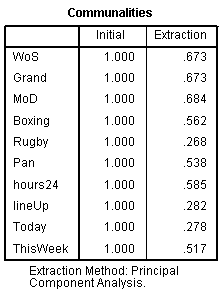
Communalities

The communalities are computations of the extent to which a variable is explained by the components. Note that Today has the lowest communality, which indicates that viewing of the Today program is less well explained by the analysis than any of the other programs (increasing the number of factors increases the communality of all the variables).

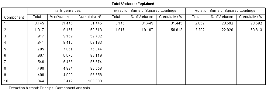
Total Variance Explained

The three right-most columns of Total Variance Explained contain the most important information on this table, and are interpreted as follows:

• Two factors (i.e., components) have been saved. That is, the analysis assumes that the 10 original variables can be reduced to 2 underlying factors. (The number of components selected has been determined by the Kaiser Rule.)
• The two components explain 51% of the variance in the data. That is, when it is assumed that there are two components, we can predict 51% of the information in all the 10 variables. (By chance, we would expect to be able to predict 2/10=20%.)
• The first component explains more of the variance than the second component (29% versus 22%).

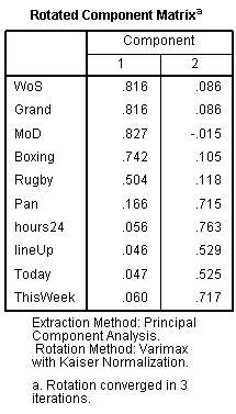
Rotated Component Matrix

The rotated component matrix, sometimes referred to as the loadings, is the key output of principal components analysis. It contains estimates of the correlations between each of the variables and the estimated components. In this example:

• There are moderate-to-strong correlations between the five sports programs and component 1.
• The correlations between the current affairs programs and the first component are very low. Typically, when interpreting a component matrix,. correlations of less than 0.3 or 0.4 are regarded as being trivial. (These correlations are commonly referred to as loadings; the correlations can also be negative and in such an instance correlations of between -0.4 or -0.3 and 0.0 are regarded as being trivially small.)
• Thus, the first component seems to measure propensity to watch sports programs.
• There are moderate-to-strong correlations between the five current affairs programs and the second component and low correlations between the sports programs and this component. Thus, the second component seems to measure propensity to watch current affairs programs.

See also

• The Basic Mechanics of Principal Components Analysis
• Saved Principal Components Analysis Variables
• Common Misinterpretations of Principal Components Analysis

Also known as

Factor Analysis (technically this is a different method, but most people that say "factor analysis" means principal components analysis).

References

Template:Reflist